DSA The Traveling Salesman Problem
The Traveling Salesman Problem
The Traveling Salesman Problem states that you are a salesperson and you must visit a number of cities or towns.
The Traveling Salesman Problem
Rules: Visit every city only once, then return back to the city you started in.
Goal: Find the shortest possible route.
Except for the Held-Karp algorithm (which is quite advanced and time consuming, (\(O(2^n n^2)\)), and will not be described here), there is no other way to find the shortest route than to check all possible routes.
This means that the time complexity for solving this problem is \(O(n!)\), which means 720 routes needs to be checked for 6 cities, 40,320 routes must be checked for 8 cities, and if you have 10 cities to visit, more than 3.6 million routes must be checked!
Note: "!", or "factorial", is a mathematical operation used in combinatorics to find out how many possible ways something can be done. If there are 4 cities, each city is connected to every other city, and we must visit every city exactly once, there are \(4!= 4 \cdot 3 \cdot 2 \cdot 1 = 24\) different routes we can take to visit those cities.
The Traveling Salesman Problem (TSP) is a problem that is interesting to study because it is very practical, but so time consuming to solve, that it becomes nearly impossible to find the shortest route, even in a graph with just 20-30 vertices.
If we had an effective algorithm for solving The Traveling Salesman Problem, the consequences would be very big in many sectors, like for example chip design, vehicle routing, telecommunications, and urban planning.
Checking All Routes to Solve The Traveling Salesman Problem
To find the optimal solution to The Traveling Salesman Problem, we will check all possible routes, and every time we find a shorter route, we will store it, so that in the end we will have the shortest route.
Good: Finds the overall shortest route.
Bad: Requires an awful lot of calculation, especially for a large amount of cities, which means it is very time consuming.
How it works:
- Check the length of every possible route, one route at a time.
- Is the current route shorter than the shortest route found so far? If so, store the new shortest route.
- After checking all routes, the stored route is the shortest one.
Such a way of finding the solution to a problem is called brute force.
Brute force is not really an algorithm, it just means finding the solution by checking all possibilities, usually because of a lack of a better way to do it.
Finding the shortest route in The Traveling Salesman Problem by checking all routes (brute force).
Progress: {{progress}}%
Route distance: {{routeDist}}
n = {{vertices}} cities
{{vertices}}!={{posRoutes}} possible routes
{{ msgDone }}The reason why the brute force approach of finding the shortest route (as shown above) is so time consuming is that we are checking all routes, and the number of possible routes increases really fast when the number of cities increases.
Example
Finding the optimal solution to the Traveling Salesman Problem by checking all possible routes (brute force):
from itertools import permutations

def calculate_distance(route, distances):
    total_distance = 0
    for i in range(len(route) - 1):
        total_distance += distances[route[i]][route[i + 1]]
    total_distance += distances[route[-1]][route[0]]
    return total_distance

def brute_force_tsp(distances):
    n = len(distances)
    cities = list(range(1, n))
    shortest_route = None
    min_distance = float('inf')

    for perm in permutations(cities):
        current_route = [0] + list(perm)
        current_distance = calculate_distance(current_route, distances)

        if current_distance < min_distance:
            min_distance = current_distance
            shortest_route = current_route

    shortest_route.append(0)
    return shortest_route, min_distance

distances = [
    [0, 2, 2, 5, 9, 3],
    [2, 0, 4, 6, 7, 8],
    [2, 4, 0, 8, 6, 3],
    [5, 6, 8, 0, 4, 9],
    [9, 7, 6, 4, 0, 10],
    [3, 8, 3, 9, 10, 0]
]

route, total_distance = brute_force_tsp(distances)
print("Route:", route)
print("Total distance:", total_distance)Using A Greedy Algorithm to Solve The Traveling Salesman Problem
Since checking every possible route to solve the Traveling Salesman Problem (like we did above) is so incredibly time consuming, we can instead find a short route by just going to the nearest unvisited city in each step, which is much faster.
Good: Finds a solution to the Traveling Salesman Problem much faster than by checking all routes.
Bad: Does not find the overall shortest route, it just finds a route that is much shorter than an average random route.
How it works:
- Visit every city.
- The next city to visit is always the nearest of the unvisited cities from the city you are currently in.
- After visiting all cities, go back to the city you started in.
This way of finding an approximation to the shortest route in the Traveling Salesman Problem, by just going to the nearest unvisited city in each step, is called a greedy algorithm.
Finding an approximation to the shortest route in The Traveling Salesman Problem by always going to the nearest unvisited neighbor (greedy algorithm).
As you can see by running this simulation a few times, the routes that are found are not completely unreasonable. Except for a few times when the lines cross perhaps, especially towards the end of the algorithm, the resulting route is a lot shorter than we would get by choosing the next city at random.
Example
Finding a near-optimal solution to the Traveling Salesman Problem using the nearest-neighbor algorithm (greedy):
def nearest_neighbor_tsp(distances):
    n = len(distances)
    visited = [False] * n
    route = [0]
    visited[0] = True
    total_distance = 0

    for _ in range(1, n):
        last = route[-1]
        nearest = None
        min_dist = float('inf')
        for i in range(n):
            if not visited[i] and distances[last][i] < min_dist:
                min_dist = distances[last][i]
                nearest = i
        route.append(nearest)
        visited[nearest] = True
        total_distance += min_dist

    total_distance += distances[route[-1]][0]
    route.append(0)
    return route, total_distance

distances = [
    [0, 2, 2, 5, 9, 3],
    [2, 0, 4, 6, 7, 8],
    [2, 4, 0, 8, 6, 3],
    [5, 6, 8, 0, 4, 9],
    [9, 7, 6, 4, 0, 10],
    [3, 8, 3, 9, 10, 0]
]

route, total_distance = nearest_neighbor_tsp(distances)
print("Route:", route)
print("Total distance:", total_distance)Other Algorithms That Find Near-Optimal Solutions to The Traveling Salesman Problem
In addition to using a greedy algorithm to solve the Traveling Salesman Problem, there are also other algorithms that can find approximations to the shortest route.
These algorithms are popular because they are much more effective than to actually check all possible solutions, but as with the greedy algorithm above, they do not find the overall shortest route.
Algorithms used to find a near-optimal solution to the Traveling Salesman Problem include:
- 2-opt Heuristic: An algorithm that improves the solution step-by-step, in each step removing two edges and reconnecting the two paths in a different way to reduce the total path length.
- Genetic Algorithm: This is a type of algorithm inspired by the process of natural selection and use techniques such as selection, mutation, and crossover to evolve solutions to problems, including the TSP.
- Simulated Annealing: This method is inspired by the process of annealing in metallurgy. It involves heating and then slowly cooling a material to decrease defects. In the context of TSP, it's used to find a near-optimal solution by exploring the solution space in a way that allows for occasional moves to worse solutions, which helps to avoid getting stuck in local minima.
- Ant Colony Optimization: This algorithm is inspired by the behavior of ants in finding paths from the colony to food sources. It's a more complex probabilistic technique for solving computational problems which can be mapped to finding good paths through graphs.
Time Complexity for Solving The Traveling Salesman Problem
To get a near-optimal solution fast, we can use a greedy algorithm that just goes to the nearest unvisited city in each step, like in the second simulation on this page.
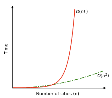
Solving The Traveling Salesman Problem in a greedy way like that, means that at each step, the distances from the current city to all other unvisited cities are compared, and that gives us a time complexity of \(O(n^2) \).
But finding the shortest route of them all requires a lot more operations, and the time complexity for that is \(O(n!)\), like mentioned earlier, which means that for 4 cities, there are 4! possible routes, which is the same as \(4 \cdot 3 \cdot 2 \cdot 1 = 24\). And for just 12 cities for example, there are \(12! = 12 \cdot 11 \cdot 10 \cdot \; ... \; \cdot 2 \cdot 1 = 479,001,600\) possible routes!
See the time complexity for the greedy algorithm \(O(n^2)\), versus the time complexity for finding the shortest route by comparing all routes \(O(n!)\), in the image below.
But there are two things we can do to reduce the number of routes we need to check.
In the Traveling Salesman Problem, the route starts and ends in the same place, which makes a cycle. This means that the length of the shortest route will be the same no matter which city we start in. That is why we have chosen a fixed city to start in for the simulation above, and that reduces the number of possible routes from \(n!\) to \((n-1)!\).
Also, because these routes go in cycles, a route has the same distance if we go in one direction or the other, so we actually just need to check the distance of half of the routes, because the other half will just be the same routes in the opposite direction, so the number of routes we need to check is actually \( \frac{(n-1)!}{2}\).
But even if we can reduce the number of routes we need to check to \( \frac{(n-1)!}{2}\), the time complexity is still \( O(n!)\), because for very big \(n\), reducing \(n\) by one and dividing by 2 does not make a significant change in how the time complexity grows when \(n\) is increased.
To better understand how time complexity works, go to this page.
Actual Traveling Salesman Problems Are More Complex
The edge weight in a graph in this context of The Traveling Salesman Problem tells us how hard it is to go from one point to another, and it is the total edge weight of a route we want to minimize.
So far on this page, the edge weight has been the distance in a straight line between two points. And that makes it much easier to explain the Traveling Salesman Problem, and to display it.
But in the real world there are many other things that affects the edge weight:
- Obstacles: When moving from one place to another, we normally try to avoid obstacles like trees, rivers, houses for example. This means it is longer and takes more time to go from A to B, and the edge weight value needs to be increased to factor that in, because it is not a straight line anymore.
- Transportation Networks: We usually follow a road or use public transport systems when traveling, and that also affects how hard it is to go (or send a package) from one place to another.
- Traffic Conditions: Travel congestion also affects the travel time, so that should also be reflected in the edge weight value.
- Legal and Political Boundaries: Crossing border for example, might make one route harder to choose than another, which means the shortest straight line route might be slower, or more costly.
- Economic Factors: Using fuel, using the time of employees, maintaining vehicles, all these things cost money and should also be factored into the edge weights.
As you can see, just using the straight line distances as the edge weights, might be too simple compared to the real problem. And solving the Traveling Salesman Problem for such a simplified problem model would probably give us a solution that is not optimal in a practical sense.
It is not easy to visualize a Traveling Salesman Problem when the edge length is not just the straight line distance between two points anymore, but the computer handles that very well.
