Excel Case: Poke Mart, Styling
Case: Poke Mart, Styling
This case is about helping the Poke Mart merchant to style the shop cart overview. You will practice the skills that you have learned in the chapters about formatting and styling.
Did you solve the first case about the Shop Cart? We will reuse that data. Check it out here.
You do not need the calculations to complete the case. Type the following data:
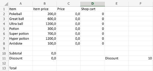
Merchant: Oh boy! I am glad that you are here to help. This colorless Shop Cart has been declining our sales. Let's give it a lift!
To complete this case you need to:
- Hide grids
- Add colors
- Change fonts
- Format numbers
- Finish the last calculation
Ready?
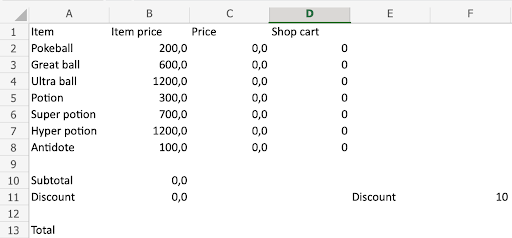
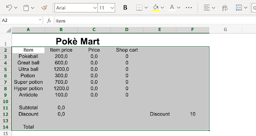
Start by removing the grids
- Click view
- Uncheck gridlines

Like this:
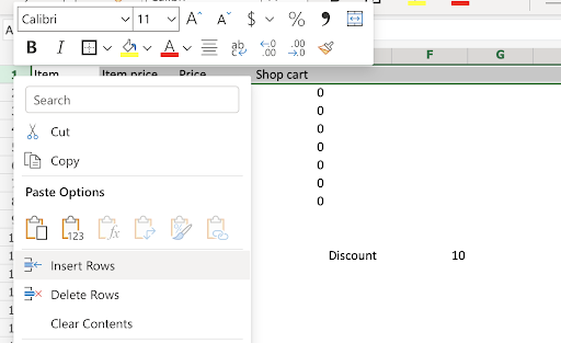
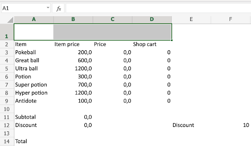
Make space for the heading by creating a new row 1.
- Right click row
1 - Insert new row

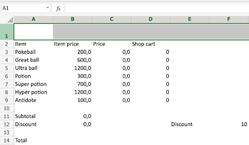
That's a start! You have created a new row 1.
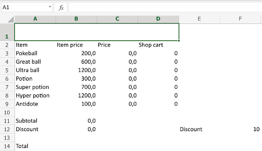
Make space for the header, increase the row height to 40 pixels.
Note: You will see the border size box which indicates the pixels when you start to drag the border.
- Drag Row 1 border to 40 pixels
Merge A1:D1 to create one big cell for the header.
- Select
A1:D1 - Click the Merge button in the Ribbon
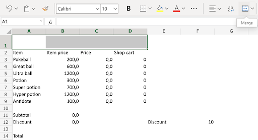
Great job! Now there is a big merged cell ready for the header.
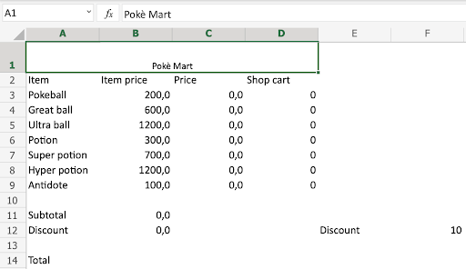
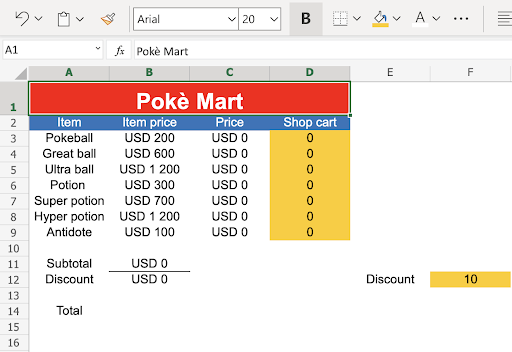
Type Poke Mart in the merged range A1:D1
- Select
A1:D1(click the merged range) - Type Poke Mart
- Hit enter
The header font is a bit small, huh?
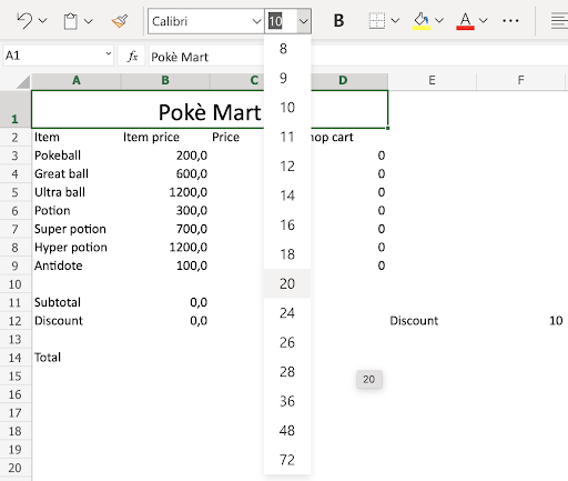
Change the header font to size 20 and make it Bold
- Select
A1:D1(the merged range) - Change to font size
20 - Click the Bold command or use keyboard shortcut CTRL + B or Command + B
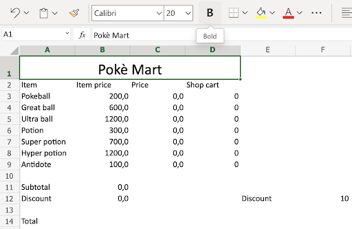
That's the way! The header looks better now.
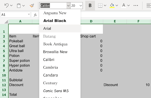
For all cells, change the font to Arial and align text for A2:F14 to Center.
- Select all cells by clicking the angle icon in the top left corner of the sheet
- Change all fonts to Arial
- Mark
A2:F14 - Click the Align button in the Ribbon
- Click the Align Center command
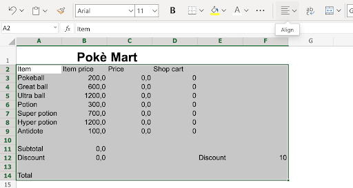
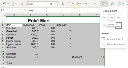
Good job! You have changed the fonts for all text to Arial and aligned A2:F14 to the Center.
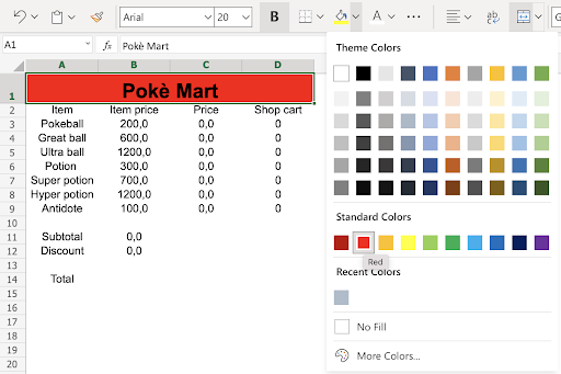
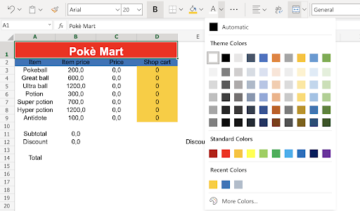
It's time to get some colors in there.
- Select range
A1:D1(the merged cells) - Apply standard Red color
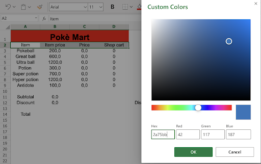
- Select
A2:D2 - Apply HEX code
2a75bb - Select
D3:D9 - Apply RGB code
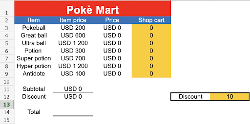
255 203 5 - Select F12
- Apply HEX code
ffcb05
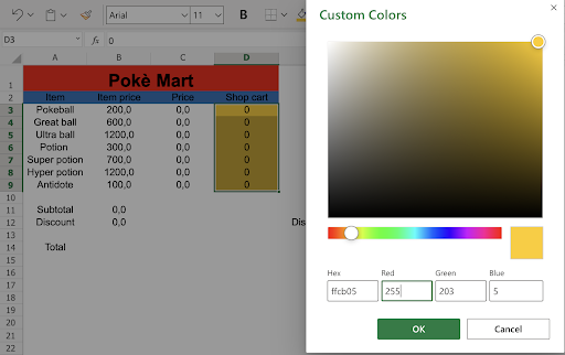
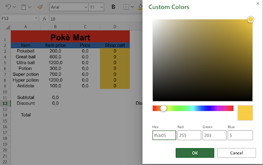
The two last colors used are the same. Same color, HEX and RGB are different.
Note: Coloring the input fields can be helpful for those who will use the spreadsheet. In this case we marked the input fields with the yellow color: ffcb05.
Next, change text colors
- Select
A1:D4 - Change text color to white
- Select
A2:A4 - Change text color to white
That is great! You got this.
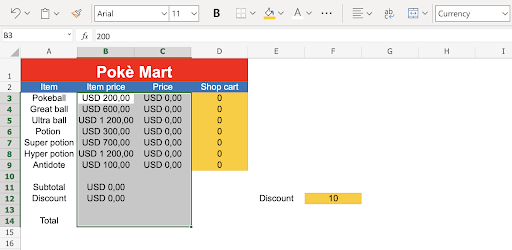
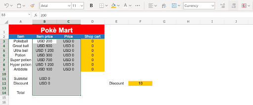
Change the Number formats for the prices to Currency and remove the decimals.
- Select
B3:C14 - Change Number format to Currency
- Click decrease decimals two times (2)

The final touch!
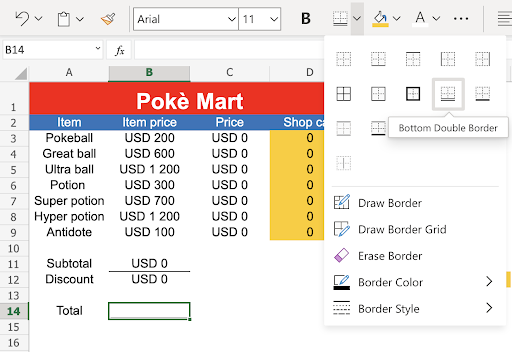
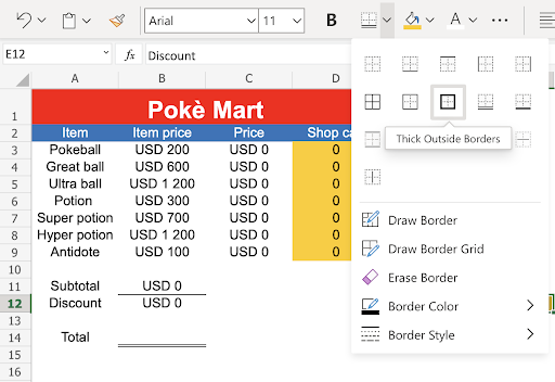
Add borders to make the numbers more readable.
B11: UnderlineB14: Double bottom borderE12:F12: Thick outside borders
- Select
B11 - Add Underline border
- Select
B14 - Add Double bottom border
- Select
E12:F12 - Add Thick outside borders
Almost there!
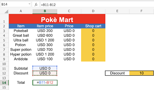
Do the final calculation for total and add the final Bold fonts.
- Select
B14 - Type
= - Select
B11 - Type
- - Select
B12 - Hit enter
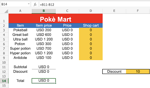
- Select
A14:B14 - Make the range bold
- Select
A2:D2 - Make the range bold
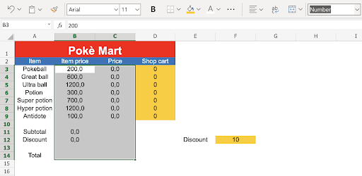
Add test values:
- Type
D3(5) - Type
D4(2) - Type
D6(5) - Type
D9(10)

Congratulations! You have successfully completed all tasks for the Poke Mart merchant.
- Hide grids - Check
- Add colors - Check
- Change fonts - Check
- Format numbers - Check
- Finish the last calculation - Check
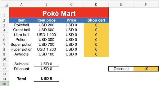
Before and After
Before styling:
After styling:
Well done!
