Excel Highlight Cell Rules
Highlight Cell Rules
Highlight Cell Rules is a premade type of conditional formatting in Excel used to change the appearance of cells in a range based on your specified conditions.
The conditions are rules based on specified numerical values, matching text, calendar dates, or duplicated and unique values.
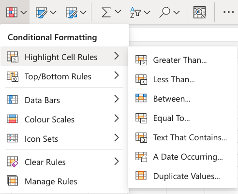
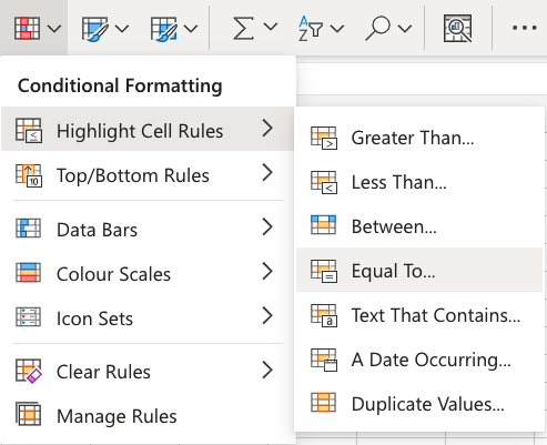
Here is the Highlight Cell Rules part of the conditional formatting menu:
Appearance Options
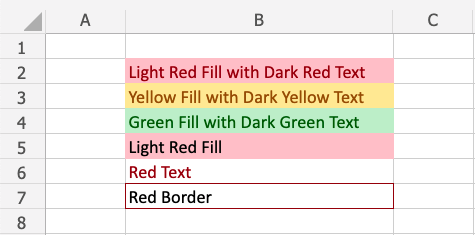
The web browser version of Excel offers the following appearance options for conditionally formatted cells:
- Light Red Fill with Dark Red Text
- Yellow Fill with Dark Yellow Text
- Green Fill with Dark Green Text
- Light Red Fill
- Red Text
- Red Border
Here is how the options look in a spreadsheet:
Cell Rule Types
Excel offers the following cell rule types:
- Greater Than...
- Less Than...
- Between...
- Equal To...
- Text That Contains...
- A Date Occurring...
- Duplicate/Unique Values
Highlight Cell Rule Example
The "Equal To..." Highlight Cell Rule will highlight a cell with one of the appearance options based on the cell value being equal to your specified value.
The specified value could be a particular number or particular text.
In this example, the specified value will be "48".
Example
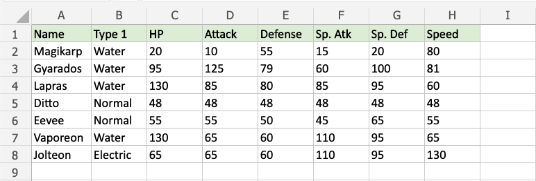
You can choose any range for where the Highlight Cell Rule should apply. It can be a few cells, a single column, a single row, or a combination of multiple cells, rows and columns.
Let's apply the rule to all of the different stat values.
"Equal To..." Highlight Cell Rule, step by step:
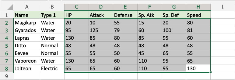
- Select the range
C2:H8for all of the stat values
- Click on the Conditional Formatting icon
 in the ribbon, from Home menu
 - Select Highlight Cell Rules from the drop-down menu
- Select Equal To... from the menu
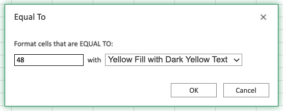
This will open a dialog box where you can specify the value and the appearance option.
- Enter
48into the input field - Select the appearance option "Yellow Fill with Dark Yellow Text" from the dropdown menu
Now, the cells with values equal to "48" will be highlighted in yellow:
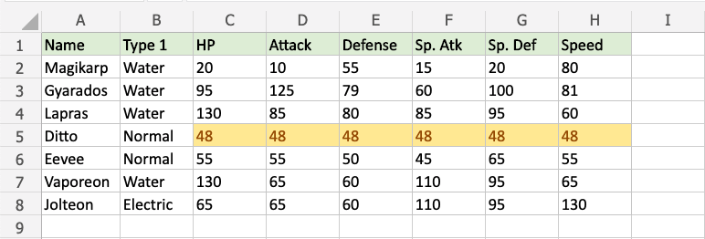
All of Ditto's stat values are 48, so they are highlighted.
Note: You can remove the Highlight Cell Rules with Manage Rules.
