Excel VLOOKUP Function
VLOOKUP Function
The VLOOKUP function is a premade function in Excel, which allows searches across columns.
It is typed =VLOOKUP and has the following parts:
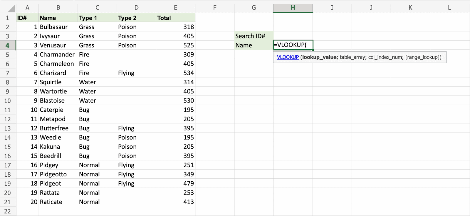
=VLOOKUP(lookup_value, table_array,
col_index_num, [range_lookup])
Note: The column which holds the data used to lookup must always be to the left.
Note: The different parts of the function are separated by a symbol, like comma , or semicolon ;
The symbol depends on your Language Settings.
Lookup_value: Select the cell where search values will be entered.
Table_array: The table range, including all cells in the table.
Col_index_num: The data which is being looked up. The input is the number of the column, counted from the left:
Range_lookup: TRUE if numbers (1) or FALSE if text (0).
Note: Both 1 / 0 and True / False can be used in Range_lookup.
How to use the VLOOKUP function.
- Select a cell (
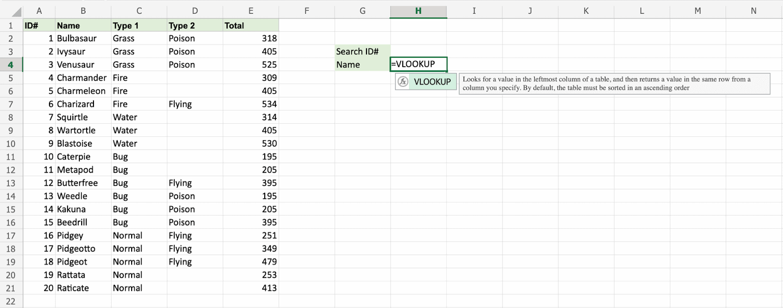
H4) - Type
=VLOOKUP - Double click the VLOOKUP command
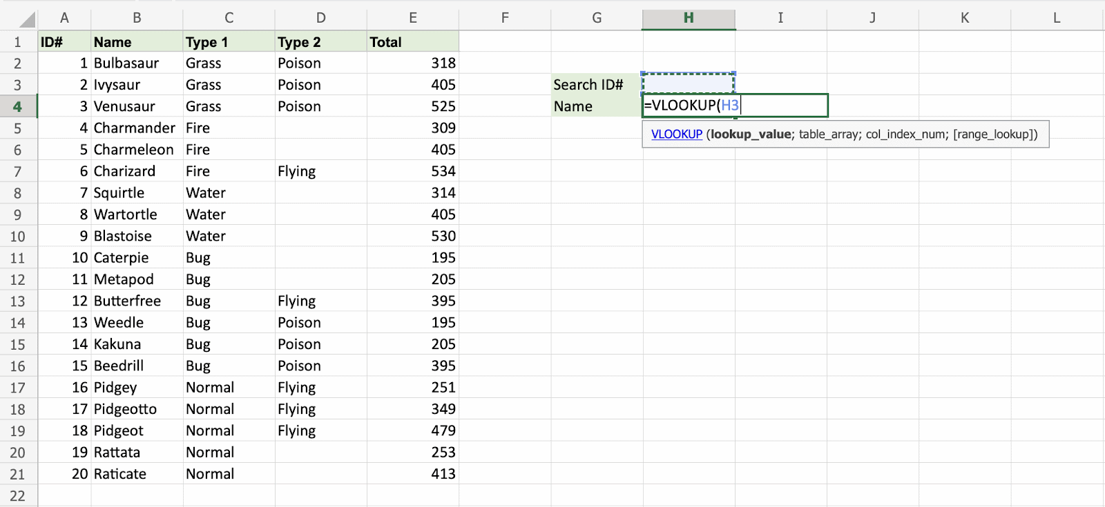
- Select the cell where search value will be entered (
H3) - Type (
,) - Mark table range (
A2:E21) - Type (
,) - Type the number of the column, counted from the left (
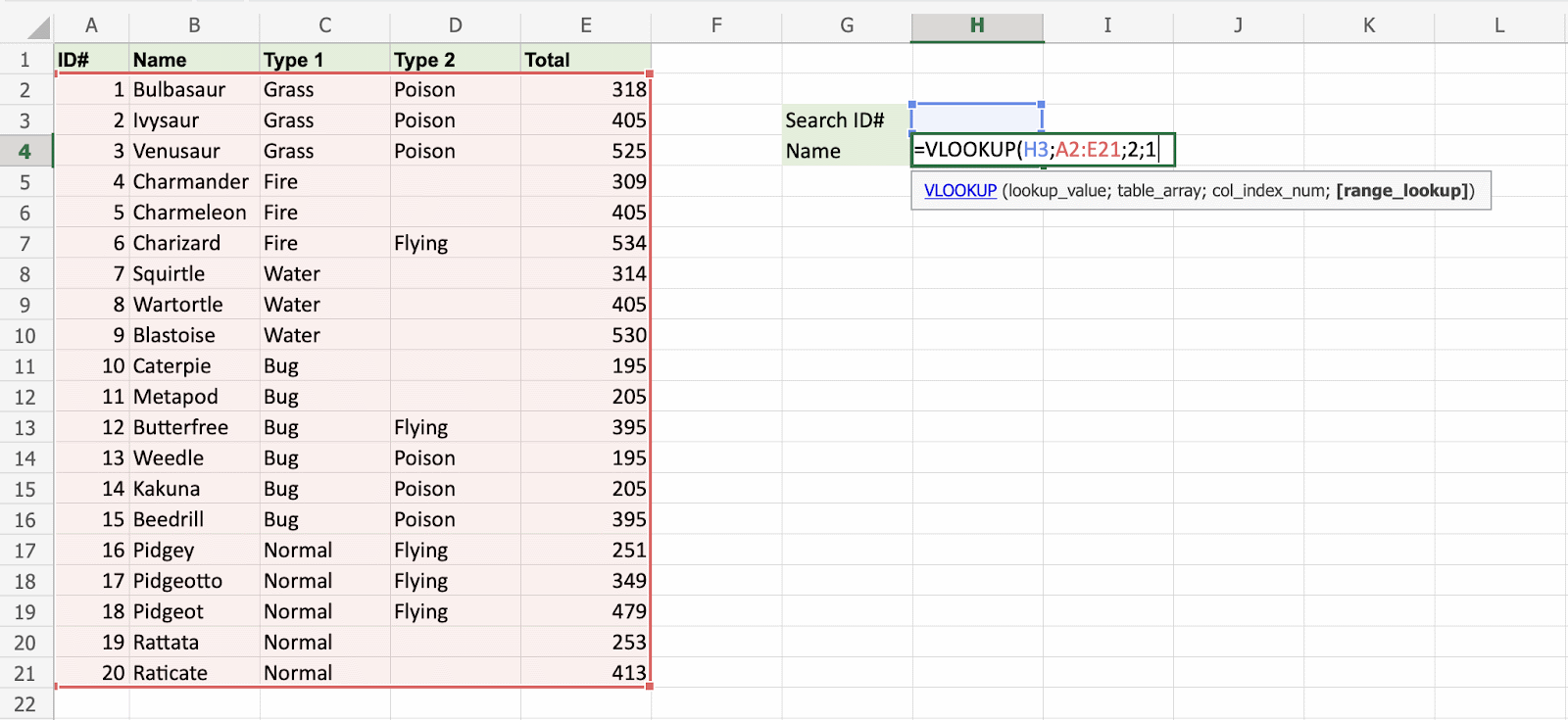
2) - Type True (1) or False (0) (
1) - Hit enter
- Enter a value in the cell selected for the Lookup_value
H3(7)
Let's have a look at an example!
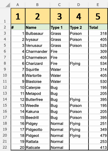
Use the VLOOKUP function to find the Pokemon names based on their ID#:
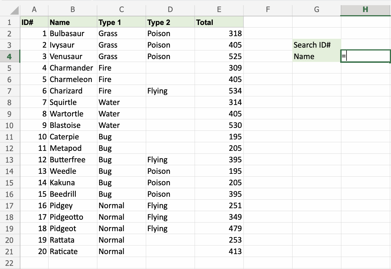
H4 is where the search result is displayed. In this case, the Pokemons names based on their ID#.
H3 selected as lookup_value. This is the cell where the search query is entered. In this case the Pokemons ID#.
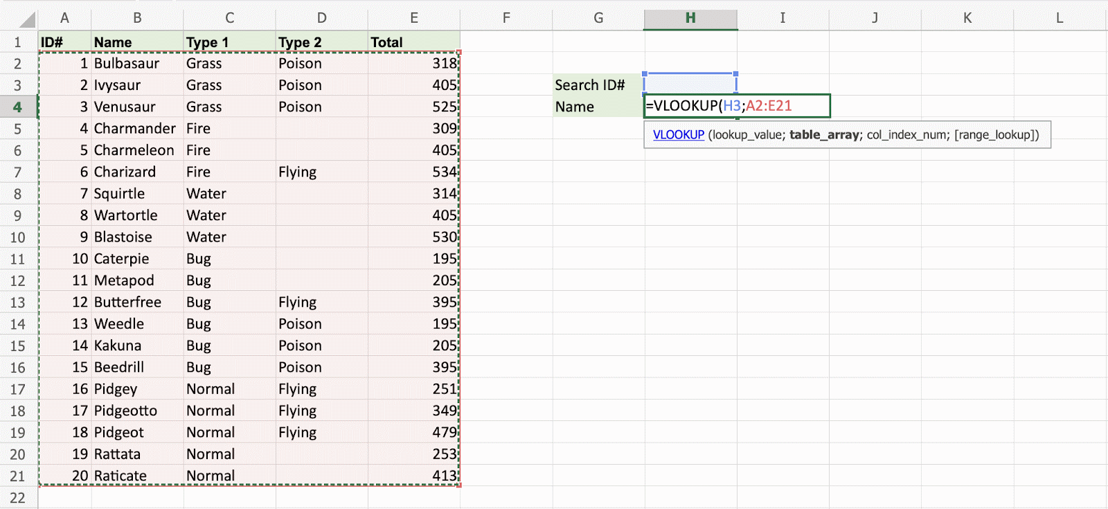
The range of the table is marked at table_array, in this example A2:E21.
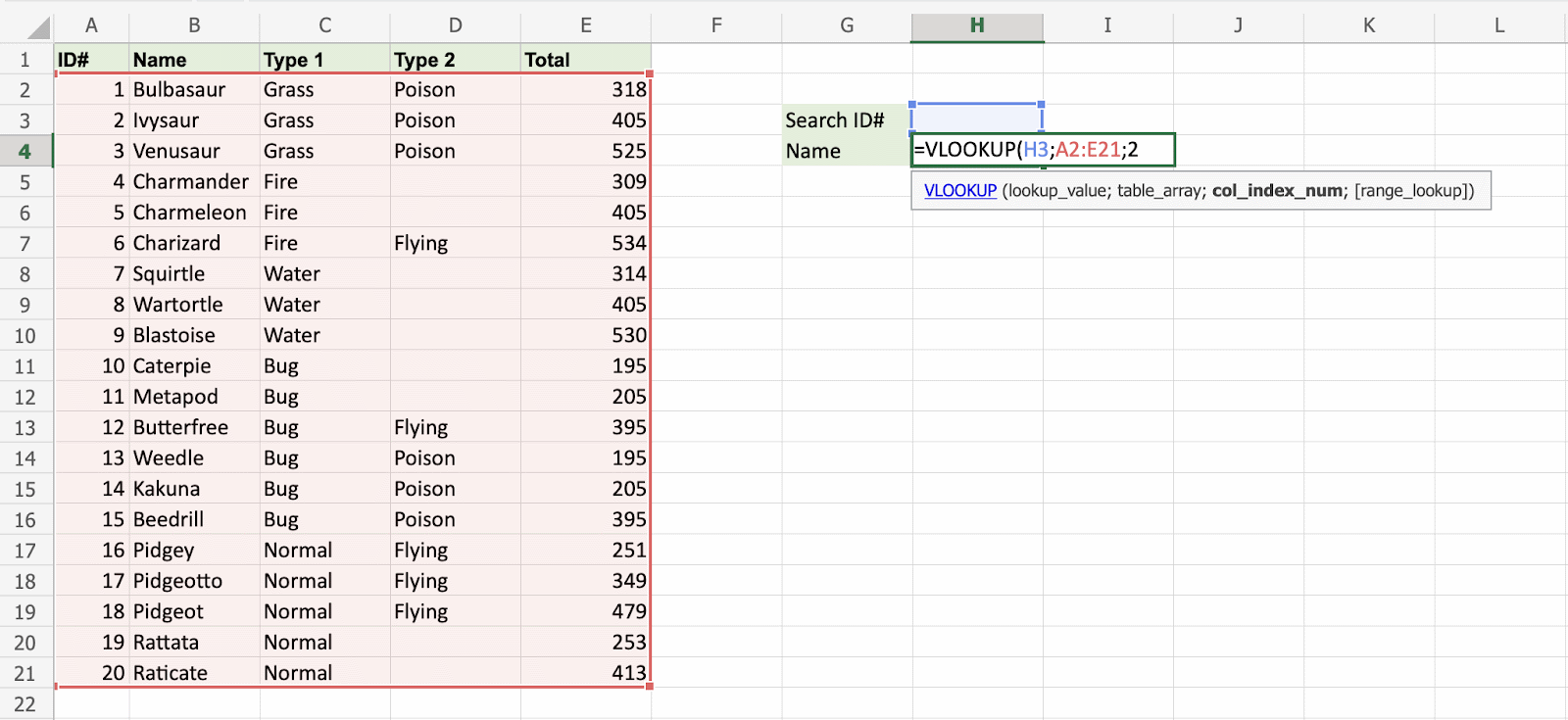
The number 2 is entered as col_index_number. This is the second column from the left and is the data that is being looked up.
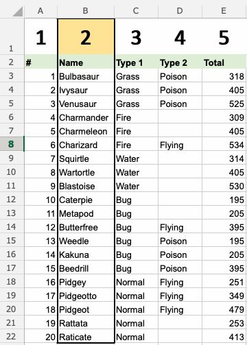
An illustration for selecting col_index_number 2.
Ok, so next - 1 (True) is entered as range_lookup. This is because the most left column has numbers only. If it was text,
0 (False) would have been used.

Good job! The function returns the #N/A value. This is because there have not been entered any value to the Search ID# H3.
Let us feed a value to it, type H3(7):
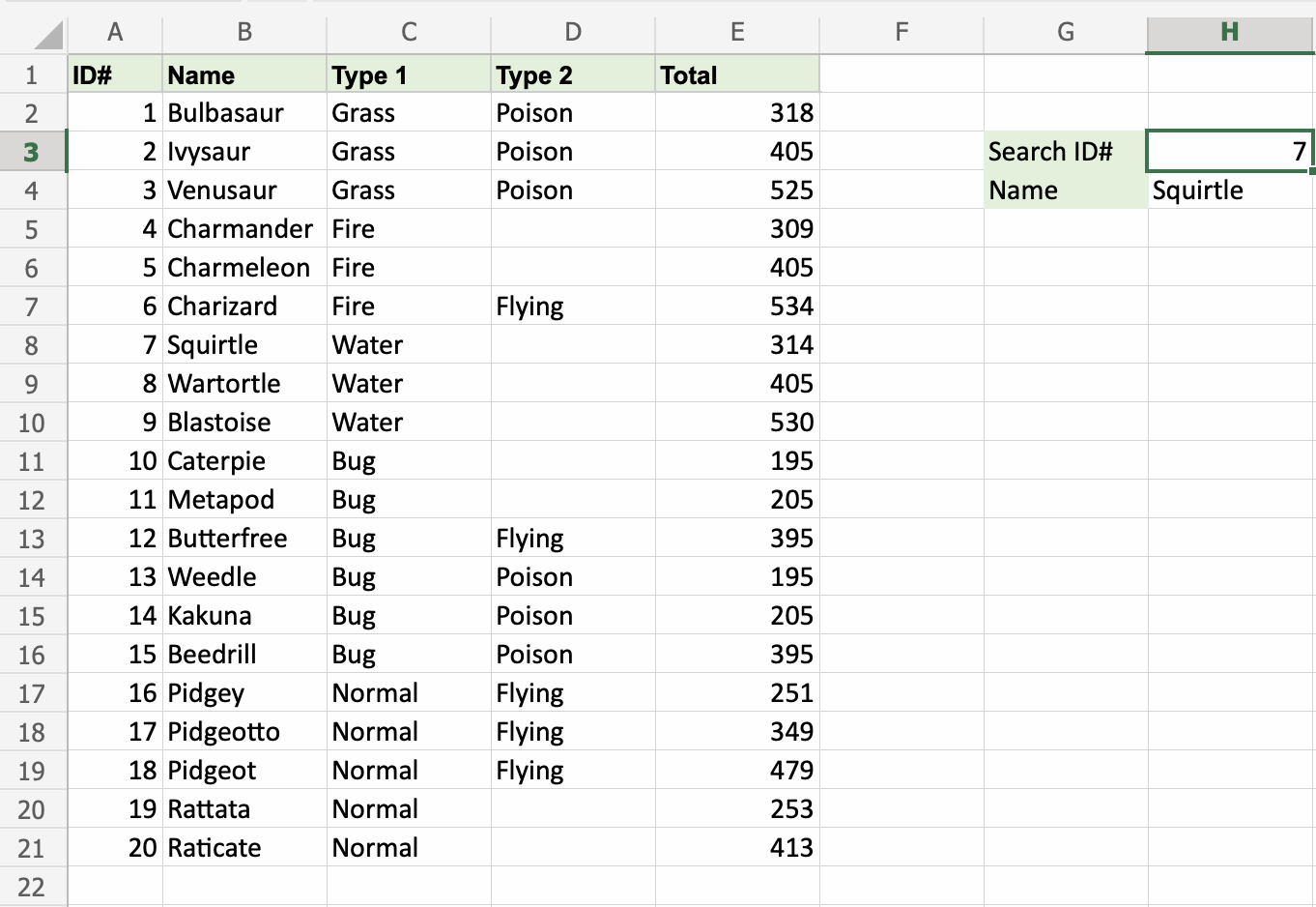
Have a look at that! The VLOOKUP function has successfully found the Pokemon Squirtle which has the ID# 7.
One more time, type (H3)4:
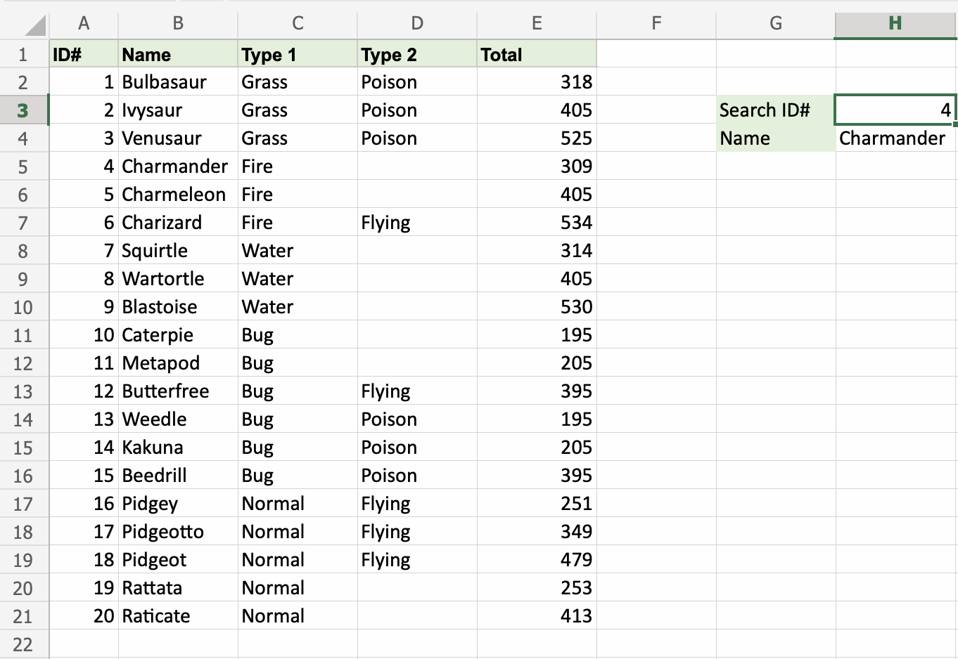
It still works! The function returned Charmanders name, which has 4 as its ID#. That's great.
