Excel Data Bars
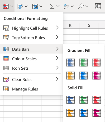
Data Bars
Data Bars are premade types of conditional formatting in Excel used to add colored bars to cells in a range to indicate how large the cell values are compared to the other values.
Here is the Data Bars part of the conditional formatting menu:
Data Bars Example
Example
You can choose any range for where the Highlight Cell Rule should apply. It can be a few cells, a single column, a single row, or a combination of multiple cells, rows and columns.
Note: The size of the data bars depends on the smallest and largest cell value in the range.
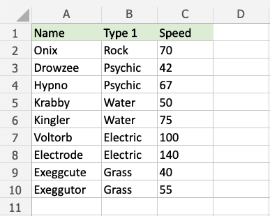
Let's apply the Data Bars conditional formatting to the Speed values.
"Data Bars", step by step:
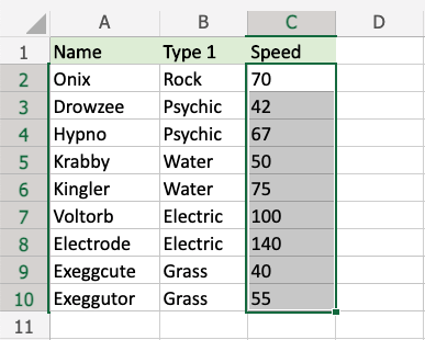
- Select the range
C2:C10for Speed values
- Click on the Conditional Formatting icon
 in the ribbon, from Home menu
 - Select Data Bars from the drop-down menu
- Select the "Green Data Bars" color option from the Gradient Fill menu
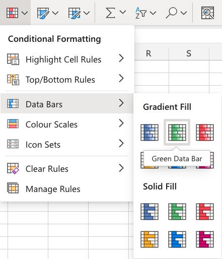
Note: Both Gradient Fill and Solid Fill work the same way. The only difference between those, and the color options are aesthetic.
Now, all of the Speed value cells have a green bar showing how big the value is compared to the other values in the range:
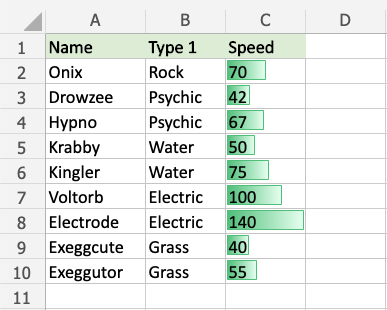
Electrode has the highest value, 140, so the bar fills the entire cell.
The other bars are scaled relative to the highest value and 0 by default.
Exeggcute has the lowest value, 40, so this is the shortest bar. Though, it is larger than 0, so there is still a small bar.
Let's see what happens if we add a fictional Pokemon with a 0 Speed value:
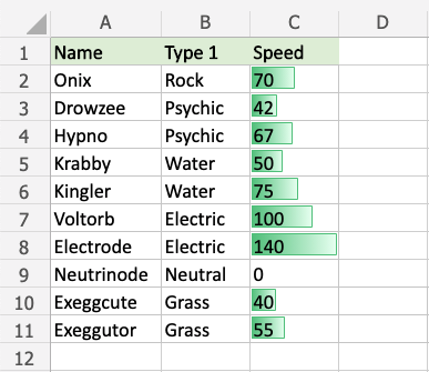
The fictional Neutrinode has a Speed value of 0, so this becomes an invisible "minimum" bar.
Let's see what happens if we add another fictional Pokemon with a negative Speed value:
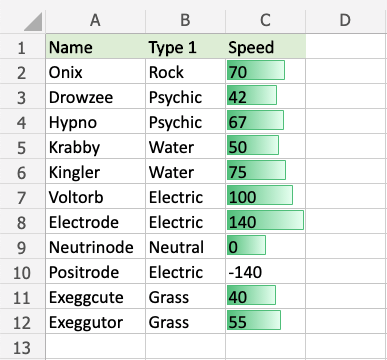
Now, the fictional Positrode has the lowest Speed value, -140, so this becomes an invisible "minimum" bar.
Notice that all the other bars have now been scaled relative to the new minimum (-140).
Neutrinode's Speed value of 0 is now in the middle between -140 and 140, so the cell has a bar filling half the cell.
Electrode still has the highest Speed value, 140, so this bar still fills the entire cell.
Note: You can remove the Highlight Cell Rules with Manage Rules.
