
Excel PivotTable Calculated Field
Calculated Field
A calculated field is a new field that you make with a formula. The formula uses the other fields, like Sales and Cost.
The new field lives in the PivotTable. The source data does not change.
This chapter uses Poke Mart sales data. Download it to follow along: poke_mart_sales.xlsx
Start with a PivotTable that has Category in Rows and Sum of Sales in Values, formatted with a thousands separator. See Create a PivotTable and PivotTable Values.
Add a Calculated Field
The data has Sales and Cost, but no Profit. Let's add it: Profit = Sales - Cost.
- Click any cell in the PivotTable
- Click PivotTable Analyze > Fields, Items, & Sets > Calculated Field
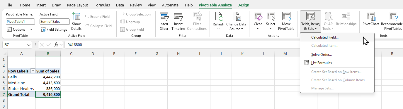
The Insert Calculated Field dialog opens.
- Type Profit in the Name box
- Delete the 0 in the Formula box
- Double-click Sales in the Fields list, type a minus sign, and double-click Cost
- Click Add, then OK
The formula is now:
= Sales - Cost
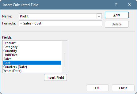
Excel adds Profit to the field list, and puts Sum of Profit in the Values area.
Format it with a thousands separator, the same way as Sum of Sales:
| A | B | C | |
|---|---|---|---|
| 3 | Row Labels | Sum of Sales | Sum of Profit |
| 4 | Balls | 4,447,200 | 1,969,640 |
| 5 | Medicine | 4,413,600 | 2,027,060 |
| 6 | Status Healers | 556,000 | 295,495 |
| 7 | Grand Total | 9,416,800 | 4,292,195 |
The Poke Mart made 4,292,195 in profit.
Excel puts "Sum of" in front of every calculated field. You can rename it in Value Field Settings, as in PivotTable Values.
Margin as a Percentage
A calculated field can use another calculated field. Let's add the margin: the share of each sale that is profit.
- Open Fields, Items, & Sets > Calculated Field again
- Name: Margin
- Formula:
= Profit / Sales - Click Add, then OK
Excel shows the margin as a decimal, like 0.442894405. To show it as a percentage:
- Open Value Field Settings for Sum of Margin
- Click Number Format and choose Percentage with 2 decimal places
- Click OK twice
| A | B | C | D | |
|---|---|---|---|---|
| 3 | Row Labels | Sum of Sales | Sum of Profit | Sum of Margin |
| 4 | Balls | 4,447,200 | 1,969,640 | 44.29% |
| 5 | Medicine | 4,413,600 | 2,027,060 | 45.93% |
| 6 | Status Healers | 556,000 | 295,495 | 53.15% |
| 7 | Grand Total | 9,416,800 | 4,292,195 | 45.58% |
Status Healers have the smallest sales, but the best margin.
Look at the Grand Total: 45.58%. That is the total profit divided by the total sales: 4,292,195 / 9,416,800.
It is not the average of the three margins above it. That is the right answer, and the next section explains why.
Calculated Fields Work on Sums
This is the most important thing to know about calculated fields.
Excel does not run the formula on each row of the data. It first sums each field for the PivotTable row, and then runs the formula on the sums.
For Balls, Margin is calculated like this: (sum of Sales - sum of Cost) / sum of Sales. That is exactly how a margin should work.
But it goes wrong for formulas that are meant to run on each row, especially with a price like UnitPrice. A sum of prices means nothing.
Correct and Incorrect
Uncheck Profit and Margin. Then add two more calculated fields:
- Revenue with the formula
= Quantity * UnitPrice(incorrect) - Avg Price with the formula
= Sales / Quantity(correct)
Format Revenue with a thousands separator, and Avg Price with 2 decimal places:
| A | B | C | D | |
|---|---|---|---|---|
| 3 | Row Labels | Sum of Sales | Sum of Revenue | Sum of Avg Price |
| 4 | Balls | 4,447,200 | 6,646,578,400 | 350.34 |
| 5 | Medicine | 4,413,600 | 6,660,055,500 | 532.08 |
| 6 | Status Healers | 556,000 | 356,373,150 | 158.90 |
| 7 | Grand Total | 9,416,800 | 34,977,434,800 | 384.55 |
Revenue is wrong. In the data, Sales is Quantity * UnitPrice on each row, so Revenue should match Sales.
Instead, Excel multiplied the total quantity for Balls (12,694) by the sum of the unit prices of all 1,035 ball orders (523,600).
The Grand Total is not even the sum of the rows above it.
Avg Price is right. Total sales divided by total items sold is the average price of one item: 4,447,200 / 12,694 = 350.34 for Balls.
Note: Do math that belongs to each row, like Quantity * UnitPrice, in a new column in the source data. Use calculated fields for math on totals, like profit, margin or average price.
Change or Delete a Calculated Field
To change a calculated field:
- Open Fields, Items, & Sets > Calculated Field
- Pick the field in the Name list, for example Margin
- Change the formula
- Click Modify, then OK
To delete it, pick it in the Name list and click Delete.
Unchecking a calculated field in the PivotTable Fields pane only takes it out of the PivotTable. It stays in the field list until you delete it.
Note: If Calculated Field is grayed out, the PivotTable probably uses the Data Model. Those PivotTables use measures instead of calculated fields.