
Excel Create a PivotTable
Create a PivotTable
A PivotTable summarizes a large table in a few clicks.
You do not write any formulas. You pick the fields you want to see, and Excel does the math.
In this chapter, you will turn 2,740 rows of Poke Mart sales into a short summary of sales by category.
This chapter uses Poke Mart sales data. Download it to follow along: poke_mart_sales.xlsx
New to PivotTables? Read the PivotTable Introduction first.
The Example Data
The file has one sheet, Sales, with one row for each order.
The data is in the range A1:J2741: one header row and 2,740 orders from 2024 and 2025.
Here are the first rows:
| A | B | C | D | E | F | G | H | I | J | |
|---|---|---|---|---|---|---|---|---|---|---|
| 1 | OrderID | Date | Store | Region | Product | Category | Quantity | UnitPrice | Sales | Cost |
| 2 | 1001 | 2024-01-01 | Lilycove City | Hoenn | Hyper Potion | Medicine | 1 | 1200 | 1200 | 680 |
| 3 | 1002 | 2024-01-01 | Cerulean City | Kanto | Poke Ball | Balls | 19 | 200 | 3800 | 2090 |
| 4 | 1003 | 2024-01-02 | Lilycove City | Hoenn | Great Ball | Balls | 13 | 600 | 7800 | 4290 |
| 5 | 1004 | 2024-01-02 | Cerulean City | Kanto | Antidote | Status Healers | 9 | 100 | 900 | 405 |
| 6 | 1005 | 2024-01-03 | Violet City | Johto | Potion | Medicine | 19 | 300 | 5700 | 2850 |
The columns are:
| Column | Description |
|---|---|
| OrderID | A unique number for each order, from 1001 to 3740 |
| Date | The order date, from 2024-01-01 to 2025-12-31 |
| Store | The Poke Mart store that made the sale. There are 6 stores |
| Region | The region of the store: Kanto, Johto or Hoenn |
| Product | The item that was sold, for example Poke Ball or Potion. There are 10 products |
| Category | The product group: Balls, Medicine or Status Healers |
| Quantity | How many items the order had |
| UnitPrice | The price of one item |
| Sales | The order total: Quantity * UnitPrice |
| Cost | What the items cost the Poke Mart |
Prepare the Data
A PivotTable needs data in a simple table shape:
- One header row, with a unique name at the top of each column
- No blank rows or blank columns inside the data
- One kind of data in each column, for example only dates in the Date column
- No merged cells, and no subtotal rows mixed in with the data
The Poke Mart data already follows these rules.
Tip: Format the Data as a Table
This step is optional, but it helps later.
Click any cell in the data and press Ctrl+T, then click OK. You can read more in Excel Tables.
A table grows by itself when you add new rows below it.
A PivotTable that uses a table picks up the new rows the next time you refresh it.
A PivotTable that uses a fixed range, like A1:J2741, does not. You would have to change the range yourself with PivotTable Analyze > Change Data Source.
Insert a PivotTable
Follow these steps:
- Click any cell in the data, for example
A1 - Click the Insert tab
- Click the PivotTable arrow, then From Table/Range
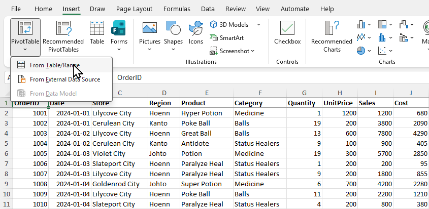
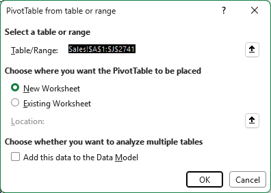
The PivotTable from table or range dialog opens.
- Check the Table/Range box. Excel fills in the whole data range for you:
Sales!$A$1:$J$2741. If you made a table, it shows the table name instead, likeTable1 - Choose New Worksheet
- Click OK
Excel adds a new sheet with an empty PivotTable. The PivotTable Fields pane opens on the right.
Note: In older versions of Excel, this dialog is called Create PivotTable. It works the same way.
The PivotTable Fields Pane
The top of the pane lists every column header from your data. In a PivotTable, the columns are called fields.
The bottom of the pane has four areas:
- Filters: filter the whole PivotTable by a field
- Columns: show each value of a field as a column
- Rows: show each value of a field as a row
- Values: the numbers to calculate, such as a sum or a count
Drag a field from the list down to an area to use it.
You can also check the box next to a field. Excel then puts text fields in Rows and number fields in Values.
To remove a field, uncheck its box, or drag it out of the area.
Note: The pane only shows when a cell inside the PivotTable is selected. If it stays hidden, click PivotTable Analyze > Field List.
Your First PivotTable
Let's find the sales for each product category.
- Drag Category to the Rows area
- Drag Sales to the Values area
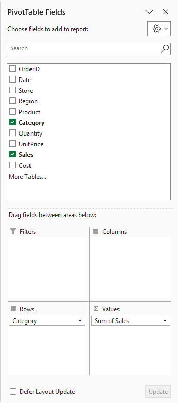
The PivotTable now looks like this:
| A | B | |
|---|---|---|
| 1 | ||
| 2 | ||
| 3 | Row Labels | Sum of Sales |
| 4 | Balls | 4447200 |
| 5 | Medicine | 4413600 |
| 6 | Status Healers | 556000 |
| 7 | Grand Total | 9416800 |
Excel adds up the Sales for each category. It calls the result Sum of Sales.
The Grand Total is the sum of all 2,740 orders: 9,416,800.
Excel places a new PivotTable in cell A3. Rows 1 and 2 stay free for the Filters area, which you will use in the Filter chapter.
The numbers have no thousands separator yet. You will format them in the Values chapter.
Good job! 2,740 rows of data became a summary of three lines.
Add a Field to Columns
Now split each category by region.
- Drag Region to the Columns area
| A | B | C | D | E | |
|---|---|---|---|---|---|
| 1 | |||||
| 2 | |||||
| 3 | Sum of Sales | Column Labels | |||
| 4 | Row Labels | Hoenn | Johto | Kanto | Grand Total |
| 5 | Balls | 1479400 | 1647600 | 1320200 | 4447200 |
| 6 | Medicine | 1303300 | 1516300 | 1594000 | 4413600 |
| 7 | Status Healers | 189300 | 199750 | 166950 | 556000 |
| 8 | Grand Total | 2972000 | 3363650 | 3081150 | 9416800 |
Each cell shows the sales of one category in one region. For example, Medicine sold 1,594,000 in Kanto (cell D6).
The Grand Total column on the right adds up each row. The Grand Total row at the bottom adds up each column.
Try dragging Region from Columns to Rows. The numbers stay the same, but the layout changes.
Moving fields between areas to look at the data from a new angle is called pivoting.
Refresh a PivotTable
A PivotTable does not update on its own when the source data changes.
After you change the data, refresh the PivotTable:
- Click any cell in the PivotTable
- Click the PivotTable Analyze tab
- Click Refresh
You can also right-click the PivotTable and choose Refresh.
Note: The PivotTable Analyze tab only appears when a cell in the PivotTable is selected. In older versions of Excel, the tab is called Analyze or Options.
If you add new rows below a fixed range, Refresh does not include them. That is why a table is the better source (see the tip above).
Recommended PivotTables
Not sure where to start? Click Insert > Recommended PivotTables, and Excel suggests ready-made PivotTables for your data that you can pick and then change.