
Excel PivotTable Filter and Slicers
Filter a PivotTable
Filters let you focus on part of the data, for example one region or the best-selling products.
The source data does not change. Only the PivotTable shows less.
This chapter uses Poke Mart sales data. Download it to follow along: poke_mart_sales.xlsx
Start with a PivotTable that has Category in Rows and Sum of Sales in Values, formatted with a thousands separator. See Create a PivotTable and PivotTable Values.
The Filters Area
A field in the Filters area filters the whole PivotTable.
Let's show the sales of the Johto region only:
- Drag Region to the Filters area
- Excel adds a filter above the PivotTable, in
A1:B1. It shows (All) - Click the arrow in
B1 - Choose Johto
- Click OK
| A | B | |
|---|---|---|
| 1 | Region | Johto |
| 2 | ||
| 3 | Row Labels | Sum of Sales |
| 4 | Balls | 1,647,600 |
| 5 | Medicine | 1,516,300 |
| 6 | Status Healers | 199,750 |
| 7 | Grand Total | 3,363,650 |
Only the Johto orders are counted now. Johto sold 3,363,650 of the 9,416,800 total.
To pick more than one region, check Select Multiple Items at the bottom of the list. The filter cell then shows (Multiple Items).
To remove the filter, choose (All) again.
Sort a PivotTable
Set the Region filter back to (All). Then uncheck Category and drag Product to the Rows area.
Excel lists the products from A to Z. To put the best sellers on top:
- Right-click any number in the Sum of Sales column
- Choose Sort > Sort Largest to Smallest
| A | B | |
|---|---|---|
| 1 | Region | (All) |
| 2 | ||
| 3 | Row Labels | Sum of Sales |
| 4 | Poke Ball | 1,821,600 |
| 5 | Great Ball | 1,677,600 |
| 6 | Super Potion | 1,545,600 |
| 7 | Potion | 1,527,000 |
| 8 | Ultra Ball | 948,000 |
| 9 | Revive | 723,000 |
| 10 | Hyper Potion | 618,000 |
| 11 | Paralyze Heal | 195,600 |
| 12 | Awakening | 180,500 |
| 13 | Antidote | 179,900 |
| 14 | Grand Total | 9,416,800 |
The Poke Ball is the best seller. The Antidote sells the least.
To sort by name again, click the arrow in A3 (Row Labels) and choose Sort A to Z.
Read more about sorting in Excel Sort.
Label Filters and Value Filters
Click the arrow in A3 (Row Labels). The menu has two kinds of filters:
- Label Filters filter by the names of the items, for example products that contain a word
- Value Filters filter by the numbers, for example the top 3 products by sales
Label Filter
Show only the products with "Potion" in the name:
- Click the arrow in
A3 - Choose Label Filters > Contains
- Type Potion
- Click OK
| A | B | |
|---|---|---|
| 3 | Row Labels | Sum of Sales |
| 4 | Super Potion | 1,545,600 |
| 5 | Potion | 1,527,000 |
| 6 | Hyper Potion | 618,000 |
| 7 | Grand Total | 3,690,600 |
The sort from before still applies.
To remove the filter, click the arrow in A3 and choose Clear Filter From "Product".
Value Filter: Top 3
Clear the label filter first. Then show the three best-selling products:
- Click the arrow in
A3 - Choose Value Filters > Top 10
- The dialog says Top 10 Items by Sum of Sales. Change 10 to 3
- Click OK
| A | B | |
|---|---|---|
| 3 | Row Labels | Sum of Sales |
| 4 | Poke Ball | 1,821,600 |
| 5 | Great Ball | 1,677,600 |
| 6 | Super Potion | 1,545,600 |
| 7 | Grand Total | 5,044,800 |
The Grand Total only adds up the items you can see: 5,044,800, not 9,416,800.
The same dialog can show the Bottom items instead, or a percent or sum of the total instead of a number of items.
Clear the filter before you go on.
Slicers
A slicer is a box of buttons that filters the PivotTable.
It is easier to use than the filter arrows, and it shows which filter is on at a glance.
Remove Region from the Filters area first. Then add a slicer for Region:
- Click any cell in the PivotTable
- Click PivotTable Analyze > Insert Slicer
- Check Region
- Click OK
- Click Johto in the slicer
To select more than one item, hold down Ctrl while you click, or turn on the Multi-Select button at the top of the slicer.
To show everything again, click the Clear Filter button in the top right corner of the slicer.
Timeline
A timeline is a slicer for dates. It needs a column with real Excel dates, like the Date column.
- Click any cell in the PivotTable
- Click PivotTable Analyze > Insert Timeline
- Check Date
- Click OK
- The timeline shows months. Click MONTHS in its top right corner and choose YEARS
- Click 2025
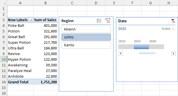
With Johto in the slicer and 2025 in the timeline, the PivotTable shows the Johto sales for 2025:
| A | B | |
|---|---|---|
| 3 | Row Labels | Sum of Sales |
| 4 | Poke Ball | 401,000 |
| 5 | Potion | 321,600 |
| 6 | Great Ball | 291,600 |
| 7 | Super Potion | 217,700 |
| 8 | Ultra Ball | 184,800 |
| 9 | Revive | 123,000 |
| 10 | Hyper Potion | 122,400 |
| 11 | Awakening | 39,500 |
| 12 | Paralyze Heal | 27,000 |
| 13 | Antidote | 22,600 |
| 14 | Grand Total | 1,751,200 |
The Date field is not in the PivotTable at all, but the timeline can still filter by it.
One slicer can also control several PivotTables that use the same data: right-click the slicer, choose Report Connections, and check the PivotTables it should filter.