
Excel PivotTable Values
PivotTable Values
The Values area decides which numbers a PivotTable shows, and how Excel calculates them.
Excel sums number fields and counts text fields by default. You can change that for each field.
This chapter uses Poke Mart sales data. Download it to follow along: poke_mart_sales.xlsx
Start with the PivotTable from the previous chapter: Category in Rows and Sum of Sales in Values.
| A | B | |
|---|---|---|
| 3 | Row Labels | Sum of Sales |
| 4 | Balls | 4447200 |
| 5 | Medicine | 4413600 |
| 6 | Status Healers | 556000 |
| 7 | Grand Total | 9416800 |
Value Field Settings
All the options for a value are in the Value Field Settings dialog. To open it:
- Click the arrow next to Sum of Sales in the Values area of the PivotTable Fields pane
- Choose Value Field Settings
You can also right-click any number in the PivotTable and choose Value Field Settings.
The dialog has four parts:
- Custom Name: the header text of the value
- Summarize Values By: how the value is calculated
- Show Values As: how the result is shown, for example as a percentage
- Number Format: how the numbers look
Summarize Values By
This tab picks the calculation. These are the ones you will use most:
| Function | What it does |
|---|---|
| Sum | Adds up the values. The default for number fields |
| Count | Counts the rows that have a value. The default for text fields |
| Average | The sum divided by the count |
| Max | The largest value |
| Min | The smallest value |
Count: Orders per Category
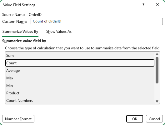
How many orders does each category have? Each order has one OrderID, so count the OrderID field.
- Drag OrderID to the Values area
- Excel shows Sum of OrderID, because OrderID is a number. Adding up order numbers makes no sense, so change it
- Open Value Field Settings for Sum of OrderID
- Choose Count and click OK
| A | B | C | |
|---|---|---|---|
| 3 | Row Labels | Sum of Sales | Count of OrderID |
| 4 | Balls | 4447200 | 1035 |
| 5 | Medicine | 4413600 | 1110 |
| 6 | Status Healers | 556000 | 595 |
| 7 | Grand Total | 9416800 | 2740 |
The header changes to Count of OrderID.
The Grand Total, 2,740, is the number of rows in the data.
Note: Count counts rows, not unique values.
For example, Count of Store shows 1035 for Balls, even though there are only 6 stores. Each of the 1,035 ball orders has a store, so each one is counted.
To count unique values, check Add this data to the Data Model when you create the PivotTable. Value Field Settings then offers Distinct Count.
Average: Sales per Order
What is the average sale per order in each category?
- Open Value Field Settings for Sum of Sales
- Choose Average and click OK
| A | B | C | |
|---|---|---|---|
| 3 | Row Labels | Average of Sales | Count of OrderID |
| 4 | Balls | 4296.811594 | 1035 |
| 5 | Medicine | 3976.216216 | 1110 |
| 6 | Status Healers | 934.4537815 | 595 |
| 7 | Grand Total | 3436.788321 | 2740 |
The header changes to Average of Sales.
The average is the sum divided by the count. For Balls: 4,447,200 / 1,035 = 4,296.81.
The Grand Total is the average of all 2,740 orders. It is not the average of the three category averages.
Excel shows many decimals here. You will learn to fix that with Number Format below.
Max and Min
Max shows the largest single value in each group. Min shows the smallest.
For example, Max of Sales shows 9600 for Balls: the biggest ball order. Min of Sales shows 1000.
Before you go on, set the Sales value back to Sum, and uncheck OrderID in the field list to remove Count of OrderID.
Show Values As
Show Values As keeps the calculation, but shows the result in a new way, for example as a percentage.
% of Grand Total
What share of all sales does each category have?
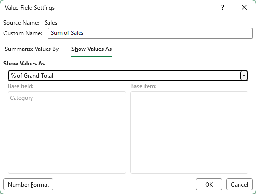
- Open Value Field Settings for Sum of Sales
- Click the Show Values As tab
- Choose % of Grand Total in the list
- Click OK
| A | B | |
|---|---|---|
| 3 | Row Labels | Sum of Sales |
| 4 | Balls | 47.23% |
| 5 | Medicine | 46.87% |
| 6 | Status Healers | 5.90% |
| 7 | Grand Total | 100.00% |
Balls and Medicine each bring in almost half of all sales. Status Healers bring in less than 6%.
The header still says Sum of Sales. The value is still a sum. It is only shown as a share of the total.
Other useful choices in the list are % of Column Total, % of Row Total and Running Total In.
To see the amounts and the percentages side by side, drag Sales to the Values area a second time, and change only the copy.
Before you go on, set Show Values As back to No Calculation.
Number Format
By default, Excel shows the sums without a thousands separator:
| A | B | |
|---|---|---|
| 3 | Row Labels | Sum of Sales |
| 4 | Balls | 4447200 |
| 5 | Medicine | 4413600 |
| 6 | Status Healers | 556000 |
| 7 | Grand Total | 9416800 |
To add a thousands separator:
- Open Value Field Settings for Sum of Sales
- Click Number Format
- Choose Number
- Set Decimal places to 0
- Check Use 1000 Separator (,)
- Click OK twice
| A | B | |
|---|---|---|
| 3 | Row Labels | Sum of Sales |
| 4 | Balls | 4,447,200 |
| 5 | Medicine | 4,413,600 |
| 6 | Status Healers | 556,000 |
| 7 | Grand Total | 9,416,800 |
Much easier to read!
The format belongs to the value field, so it stays when you rearrange or refresh the PivotTable.
If you format the cells from the Home tab instead, the format can get lost when the PivotTable changes.
Read more about number formats in Excel Format Numbers.
Rename a Value Field
You can give a value a shorter or clearer name, like Total Sales.
- Open Value Field Settings for Sum of Sales
- Type Total Sales in the Custom Name box
- Click OK
You can also click the header cell, B3, type the new name, and press Enter.
| A | B | |
|---|---|---|
| 3 | Row Labels | Total Sales |
| 4 | Balls | 4,447,200 |
| 5 | Medicine | 4,413,600 |
| 6 | Status Healers | 556,000 |
| 7 | Grand Total | 9,416,800 |
Note: A value cannot have the same name as a field in the data. If you type Sales, Excel says that the field name already exists. Pick another name, or add a space at the end of it.