
Excel PivotTable Group
Group Data in a PivotTable
Grouping combines many small items into a few bigger ones.
For example, you can group days into years and quarters, or order sizes into ranges like 1-5 and 6-10.
This chapter uses Poke Mart sales data. Download it to follow along: poke_mart_sales.xlsx
Start with a PivotTable that has Sum of Sales in Values, formatted with a thousands separator, and nothing in Rows or Columns. See Create a PivotTable and PivotTable Values.
Group Dates
The data has orders on 731 different days. One row per day would be far too long to read.
Let's group the dates into years and quarters:
- Drag Date to the Rows area
- Right-click any date in the PivotTable and choose Group. You can also click PivotTable Analyze > Group Field
- The Grouping dialog opens. Under By, click Quarters and Years so that both are selected, and click any other selected item to turn it off
- Click OK
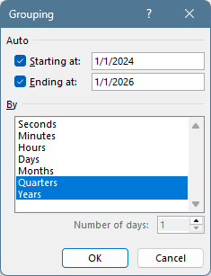
Note: Recent versions of Excel may group a date field automatically when you add it to Rows. You then see years and extra fields like Quarters in the Rows area, without opening the dialog. You can still open the Grouping dialog to change the grouping.
| A | B | |
|---|---|---|
| 3 | Row Labels | Sum of Sales |
| 4 | 2024 | 4,393,200 |
| 5 | Qtr1 | 852,950 |
| 6 | Qtr2 | 1,119,400 |
| 7 | Qtr3 | 1,223,600 |
| 8 | Qtr4 | 1,197,250 |
| 9 | 2025 | 5,023,600 |
| 10 | Qtr1 | 977,950 |
| 11 | Qtr2 | 1,197,800 |
| 12 | Qtr3 | 1,452,100 |
| 13 | Qtr4 | 1,395,750 |
| 14 | Grand Total | 9,416,800 |
Each year shows its total, with the four quarters below it.
Sales grew from 2024 to 2025, and the third quarter (Qtr3) was the best quarter in both years.
Click the minus button next to a year to collapse it, and the plus button to expand it again.
Months
Select Months in the Grouping dialog as well, and each quarter gets its months below it: Jan, Feb, Mar and so on.
For example, December 2025 was the best month of 2025, with 634,000 in sales.
Group Numbers
You can also group numbers into ranges. Let's see how big the orders are.
- Remove Date from the Rows area
- Drag Quantity to the Rows area. Drag it, because checking the box would put it in Values
- Drag OrderID to the Values area and change it to Count (see PivotTable Values)
The PivotTable now has one row for each quantity, from 1 to 30. Group them in steps of 5:
- Right-click any quantity in the PivotTable and choose Group
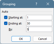
- Set Starting at to 1, Ending at to 30 and By to 5
- Click OK
| A | B | C | |
|---|---|---|---|
| 3 | Row Labels | Sum of Sales | Count of OrderID |
| 4 | 1-5 | 2,496,950 | 1041 |
| 5 | 6-10 | 3,149,750 | 883 |
| 6 | 11-15 | 1,725,400 | 388 |
| 7 | 16-20 | 1,050,900 | 233 |
| 8 | 21-25 | 449,200 | 98 |
| 9 | 26-30 | 544,600 | 97 |
| 10 | Grand Total | 9,416,800 | 2740 |
Most orders are small: 1,041 of the 2,740 orders had 5 items or fewer.
But the orders with 6 to 10 items brought in the most sales.
Group Selected Items
You can also make your own groups by picking items.
Say you want to compare Kanto with the two other regions together. Remove Quantity and Count of OrderID, and drag Region to Rows:
| A | B | |
|---|---|---|
| 3 | Row Labels | Sum of Sales |
| 4 | Hoenn | 2,972,000 |
| 5 | Johto | 3,363,650 |
| 6 | Kanto | 3,081,150 |
| 7 | Grand Total | 9,416,800 |
- Click Hoenn (
A4) - Hold down Ctrl and click Johto (
A5) - Click PivotTable Analyze > Group Selection. You can also right-click and choose Group
| A | B | |
|---|---|---|
| 3 | Row Labels | Sum of Sales |
| 4 | Group1 | 6,335,650 |
| 5 | Hoenn | 2,972,000 |
| 6 | Johto | 3,363,650 |
| 7 | Kanto | 3,081,150 |
| 8 | Kanto | 3,081,150 |
| 9 | Grand Total | 9,416,800 |
Excel adds a new field, Region2, to the Rows area.
Hoenn and Johto are now in a group called Group1. Kanto was not selected, so it gets a group of its own, also called Kanto.
Give the group a better name: click A4, type Hoenn and Johto, and press Enter.
Then right-click the group and choose Expand/Collapse > Collapse Entire Field to hide the regions inside the groups:
| A | B | |
|---|---|---|
| 3 | Row Labels | Sum of Sales |
| 4 | Hoenn and Johto | 6,335,650 |
| 5 | Kanto | 3,081,150 |
| 6 | Grand Total | 9,416,800 |
Ungroup
To remove a group, click it and choose PivotTable Analyze > Ungroup. You can also right-click it and choose Ungroup.
For grouped dates or numbers, right-click any of the groups and choose Ungroup. This removes the grouping from the whole field.
Note: If Excel says "Cannot group that selection", the field probably has blank cells or text in it. Every cell in a date column must be a real date, and every cell in a number column must be a number.