
Power BI Power Query Unpivot
Wide and Long Tables
The Poke Mart managers set a sales target for every store and every month of 2025. They keep the targets in an Excel file:
Download poke_mart_targets_2025.xlsx
The sheet Targets has one row per store and one column per month:
| A | B | C | D | E | F | G | H | I | J | K | L | M | N | |
|---|---|---|---|---|---|---|---|---|---|---|---|---|---|---|
| 1 | Region | Store | Jan | Feb | Mar | Apr | May | Jun | Jul | Aug | Sep | Oct | Nov | Dec |
| 2 | Kanto | Viridian City | 51000 | 65000 | 75000 | 87000 | 45000 | 88000 | 62000 | 70000 | 54000 | 55000 | 43000 | 158000 |
| 3 | Cerulean City | 52000 | 50000 | 72000 | 41000 | 71000 | 68000 | 78000 | 135000 | 69000 | 89000 | 101000 | 76000 | |
| 4 | Johto | Goldenrod City | 104000 | 55000 | 104000 | 95000 | 109000 | 107000 | 145000 | 179000 | 77000 | 81000 | 110000 | 141000 |
| 5 | Violet City | 25000 | 34000 | 41000 | 33000 | 61000 | 46000 | 95000 | 48000 | 41000 | 45000 | 44000 | 72000 | |
| 6 | Hoenn | Slateport City | 59000 | 54000 | 77000 | 86000 | 75000 | 77000 | 79000 | 91000 | 53000 | 56000 | 92000 | 144000 |
| 7 | Lilycove City | 53000 | 55000 | 31000 | 45000 | 88000 | 71000 | 93000 | 110000 | 91000 | 65000 | 39000 | 95000 |
This layout is called a wide table.
It is easy for people to read, but hard to analyze:
- There is no Month column, so you cannot put the month on a chart axis or in a slicer.
- To get the total target, you have to add up 12 separate columns.
- To compare targets with actual sales month by month, both tables need a month field.
- When months are added, for example for 2026, each one is a new column, and every visual that uses the months must be changed.
Power BI works best with a long table: one row for each store and month, with the month in its own column:
| ABCRegion | ABCStore | ABCMonth | 123Target |
|---|---|---|---|
| Kanto | Viridian City | Jan | 51000 |
| Kanto | Viridian City | Feb | 65000 |
| Kanto | Viridian City | Mar | 75000 |
| ... | ... | ... | ... |
6 stores times 12 months gives 72 rows.
Turning columns into rows like this is called unpivoting.
Load the Targets File
This page continues the cleanup from Replace Values and Fill Down.
Open pq_cleanup.pbix, the report you saved there, and select Home > Transform data.
Add the targets file as a new query, next to the 2024 sales:
- On the Home tab, select New Source > Excel Workbook.
- Find poke_mart_targets_2025.xlsx and select Open.
- In the Navigator, select Targets, and then select OK.
A new query called Targets appears in the Queries pane.
Power Query uses the first row as column headers and sets the data types, just as it did for the CSV file:
| ABCRegion | ABCStore | 123Jan | 123Feb | 123Mar | 123Apr | 123May | 123Jun | 123Jul | 123Aug | 123Sep | 123Oct | 123Nov | 123Dec |
|---|---|---|---|---|---|---|---|---|---|---|---|---|---|
| Kanto | Viridian City | 51000 | 65000 | 75000 | 87000 | 45000 | 88000 | 62000 | 70000 | 54000 | 55000 | 43000 | 158000 |
| null | Cerulean City | 52000 | 50000 | 72000 | 41000 | 71000 | 68000 | 78000 | 135000 | 69000 | 89000 | 101000 | 76000 |
| Johto | Goldenrod City | 104000 | 55000 | 104000 | 95000 | 109000 | 107000 | 145000 | 179000 | 77000 | 81000 | 110000 | 141000 |
| null | Violet City | 25000 | 34000 | 41000 | 33000 | 61000 | 46000 | 95000 | 48000 | 41000 | 45000 | 44000 | 72000 |
| Hoenn | Slateport City | 59000 | 54000 | 77000 | 86000 | 75000 | 77000 | 79000 | 91000 | 53000 | 56000 | 92000 | 144000 |
| null | Lilycove City | 53000 | 55000 | 31000 | 45000 | 88000 | 71000 | 93000 | 110000 | 91000 | 65000 | 39000 | 95000 |
The query has 6 rows and 14 columns.
The empty Region cells are null.
Step 1: Fill Down the Region
First fill the empty Region cells, as you learned in Replace Values and Fill Down:
- Select the Region column.
- On the Transform tab, select Fill > Down.
| ABCRegion | ABCStore | 123Jan | ... |
|---|---|---|---|
| Kanto | Viridian City | 51000 | ... |
| Kanto | Cerulean City | 52000 | ... |
| Johto | Goldenrod City | 104000 | ... |
| Johto | Violet City | 25000 | ... |
| Hoenn | Slateport City | 59000 | ... |
| Hoenn | Lilycove City | 53000 | ... |
Do this before you unpivot.
The unpivot copies each store's Region onto 12 rows, one for each month.
Without Fill Down, 36 of the 72 rows would have no region.
Step 2: Unpivot Other Columns
- Select the Region column header.
- Hold down Ctrl and select the Store column header. Both columns are now selected.
- On the Transform tab, select the arrow next to Unpivot Columns, and then select Unpivot Other Columns. The command is also on the right-click menu of the selected headers.
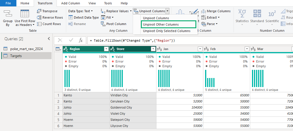
Power Query keeps Region and Store as they are, and turns the 12 month columns into two new columns:
- Attribute holds the old column names: Jan, Feb, and so on to Dec.
- Value holds the numbers that were under them.
| ABCRegion | ABCStore | ABCAttribute | 123Value |
|---|---|---|---|
| Kanto | Viridian City | Jan | 51000 |
| Kanto | Viridian City | Feb | 65000 |
| Kanto | Viridian City | Mar | 75000 |
| Kanto | Viridian City | Apr | 87000 |
| Kanto | Viridian City | May | 45000 |
| Kanto | Viridian City | Jun | 88000 |
| ... | ... | ... | ... |
| Hoenn | Lilycove City | Dec | 95000 |
The query now has 72 rows and 4 columns.
Step 3: Rename the New Columns
- Double-click the Attribute header, type
Month, and press Enter. - Double-click the Value header, type
Target, and press Enter.
| ABCRegion | ABCStore | ABCMonth | 123Target |
|---|---|---|---|
| Kanto | Viridian City | Jan | 51000 |
| Kanto | Viridian City | Feb | 65000 |
| Kanto | Viridian City | Mar | 75000 |
| Kanto | Viridian City | Apr | 87000 |
| Kanto | Viridian City | May | 45000 |
| Kanto | Viridian City | Jun | 88000 |
| ... | ... | ... | ... |
| Hoenn | Lilycove City | Dec | 95000 |
Target should be a whole number column, with the 123 icon in its header.
If your Target column shows ABC123 instead, select the icon and choose Whole Number.
Check the Totals
Unpivoting only moves numbers around.
It must not change the total.
The 72 targets must add up to 5,426,000, the same as the 72 number cells in the original sheet.
You can check the total in Power Query:
- Select the Target column.
- On the Transform tab, select Statistics > Sum. The preview now shows one number: 5426000. The new step is called Calculated Sum.
- Delete the Calculated Sum step with the X next to it in Applied Steps, so the query returns the 72 rows again.
Once the data is loaded into the report, a table visual of Target by Region shows these values:
| Region | Target |
|---|---|
| Hoenn | 1,779,000 |
| Johto | 1,892,000 |
| Kanto | 1,755,000 |
| Total | 5,426,000 |
Power BI shows these numbers without thousands separators, for example 1779000.
Unpivot and Pivot Commands
The Transform tab has three unpivot commands, and one command for the opposite direction:
| Command | What it does |
|---|---|
| Unpivot Columns | You select the columns to turn into rows (here: Jan to Dec). |
| Unpivot Other Columns | You select the columns to keep (here: Region and Store). All the other columns are turned into rows. |
| Unpivot Only Selected Columns | Like Unpivot Columns, but only exactly the columns you selected. Columns added to the source later stay as they are. |
| Pivot Column | The opposite of unpivot: the values of one column become new column headers. Pivoting Month with the values from Target gives back the wide table. |
Unpivot Other Columns is the best choice here.
You name only the two columns that stay, and if next year's file has more month columns, they are unpivoted too.
Pivot Column does what an Excel PivotTable does with a field in the Columns area: it spreads the values of one field across columns.
Unpivot goes back the other way.
The Targets query is ready.
Select Close & Apply, then File > Save to save pq_cleanup.pbix.
In the next chapter you go back to the sales data and add the 2025 orders.