
Power BI Conditional Formatting
What Is Conditional Formatting?
Conditional formatting changes the look of a value based on the value itself.
A low margin turns red.
A big sales number gets a darker cell.
It works much like conditional formatting in Excel.
In Power BI you use it mostly in tables and matrices, but chart colors can use it too.
There are five kinds of conditional formatting for tables and matrices:
| Kind | What it does |
|---|---|
| Background color | Colors the cell |
| Font color | Colors the text |
| Data bars | Draws a bar in the cell. The longer the bar, the bigger the value. |
| Icons | Adds an icon, such as a colored circle or an arrow |
| Web URL | Turns the value into a link |
Colors can be set in three ways, called format styles: Gradient (a color scale), Rules (a color for each range of values), and Field value (the color comes from a measure).
The Example Table
Work in your file from the DAX chapter, for example poke_mart_dax.pbix (see Power BI Visuals for what it holds).
The table uses the measures Total Sales, Units Sold and Margin %.
Later on this page you add one more measure, Margin Color.
- Click an empty spot on the canvas and select Table.
- Add Product from the Products table, and then Total Sales, Units Sold and Margin %.
- Select the Total Sales column header until the table is sorted from the highest to the lowest value.
This is the table, before any formatting:
| Product | Total Sales | Units Sold | Margin % |
|---|---|---|---|
| Poke Ball | 1,821,600 | 9,108 | 45.00% |
| Great Ball | 1,677,600 | 2,796 | 45.00% |
| Super Potion | 1,545,600 | 2,208 | 45.71% |
| Potion | 1,527,000 | 5,090 | 50.00% |
| Ultra Ball | 948,000 | 790 | 41.67% |
| Revive | 723,000 | 482 | 40.00% |
| Hyper Potion | 618,000 | 515 | 43.33% |
| Paralyze Heal | 195,600 | 978 | 52.50% |
| Awakening | 180,500 | 722 | 52.00% |
| Antidote | 179,900 | 1,799 | 55.00% |
| Total | 9,416,800 | 24,488 | 45.58% |
You open conditional formatting from the field itself.
In the Visualizations pane, right-click a field in the Columns well (or select the arrow next to it), and select Conditional formatting.
Background Color Scale
A color scale colors each cell by its size: light for small values, dark for big values.
It works like color scales in Excel.
- Right-click Total Sales in the Columns well and select Conditional formatting > Background color.
- Set Format style to Gradient.
- Under What field should we base this on?, make sure Total Sales is selected.
- Set Minimum to Lowest value and pick white in the color box next to it. Set Maximum to Highest value and pick a green, for example #04AA6D: in the color box, select More colors... and type 04AA6D in the Hex box.
- Select OK.
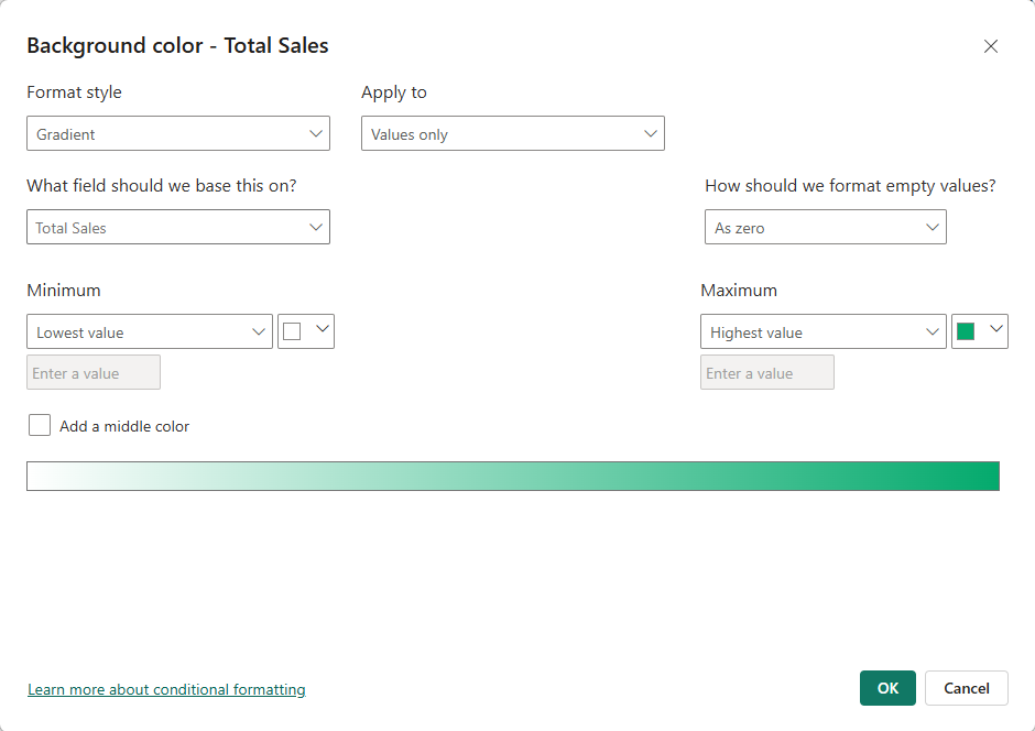
Power BI puts each value on a scale from the lowest (Antidote, 179,900) to the highest (Poke Ball, 1,821,600).
The position on the scale decides the shade:
| Product | Total Sales | Position on the scale | Shade (approximate) |
|---|---|---|---|
| Poke Ball | 1,821,600 | 100% | Full green |
| Great Ball | 1,677,600 | 91% | |
| Super Potion | 1,545,600 | 83% | |
| Potion | 1,527,000 | 82% | |
| Ultra Ball | 948,000 | 47% | About halfway |
| Revive | 723,000 | 33% | |
| Hyper Potion | 618,000 | 27% | |
| Paralyze Heal | 195,600 | 1% | Almost white |
| Awakening | 180,500 | 0% | Almost white |
| Antidote | 179,900 | 0% | White |
The position is (value - lowest) / (highest - lowest).
For Ultra Ball: (948,000 - 179,900) / (1,821,600 - 179,900) = 47%, so its cell is about halfway between white and green.
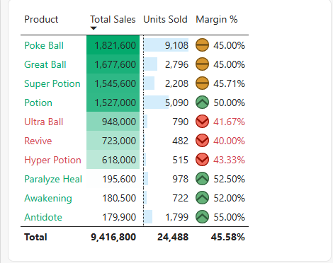
The top four products are all dark, and the three Status Healers are all white.
The scale makes the gap between the two groups easy to see.
Font Color Rules
A rule gives one color to every value in a range.
Here: show a margin below 45% in red.
- Right-click Margin % and select Conditional formatting > Font color.
- Set Format style to Rules.
- Fill in the rule: If value >= 0 Number and < 0.45 Number, then red (for example #D64550, with More colors... and the Hex box). The two unit boxes start as Percent: change both to Number.
- Select OK.
Three products turn red:
| Product | Margin % | Font color |
|---|---|---|
| Antidote | 55.00% | Default |
| Paralyze Heal | 52.50% | Default |
| Awakening | 52.00% | Default |
| Potion | 50.00% | Default |
| Super Potion | 45.71% | Default |
| Poke Ball | 45.00% | Default |
| Great Ball | 45.00% | Default |
| Hyper Potion | 43.33% | Red |
| Ultra Ball | 41.67% | Red |
| Revive | 40.00% | Red |
Poke Ball and Great Ball have a margin of exactly 45.00%.
The rule says "less than 0.45", so they stay in the default color.
Use <= in the rule if 45% should also be red.
Note: For percentages, type the real decimal value (0.45, not 45) and choose Number, not Percent.
Percent means a percent of the range between the lowest and the highest value in the column, not the value itself.
This is what goes wrong with Percent.
The margins run from 40.00% to 55.00%.
A rule "< 45 Percent" then means "in the lowest 45% of that range", which is below 40% + 0.45 × 15% = 46.75%:
| Rule | Border | Red products |
|---|---|---|
| < 0.45 Number | 45.00% | 3 |
| < 45 Percent | 46.75% | 6 |
With Percent, Super Potion, Poke Ball and Great Ball turn red too, although their margin is not below 45%.
Data Bars
Data bars draw a bar inside each cell, like data bars in Excel.
The longer the bar, the bigger the value.
- Right-click Units Sold and select Conditional formatting > Data bars.
- Leave Show bar only unchecked, so the numbers stay visible next to the bars.
- Select OK.
The bars rank the products by units, which is a different order than the sales order of the table:
| Bar length | Product | Units Sold |
|---|---|---|
| 1 (longest) | Poke Ball | 9,108 |
| 2 | Potion | 5,090 |
| 3 | Great Ball | 2,796 |
| 4 | Super Potion | 2,208 |
| 5 | Antidote | 1,799 |
| 6 | Paralyze Heal | 978 |
| 7 | Ultra Ball | 790 |
| 8 | Awakening | 722 |
| 9 | Hyper Potion | 515 |
| 10 (shortest) | Revive | 482 |
Antidote is near the bottom of the table, but its bar is the fifth longest.
It sells many units at a low price.
Icons
Icons sort values into groups at a glance, like icon sets in Excel.
Here: a green, yellow or red circle for the margin.
- Right-click Margin % and select Conditional formatting > Icons.
- Set Format style to Rules.
- Keep Icon layout at Left of data, the default, so the icon shows to the left of the value.
- Under Style, choose the set of red, yellow and green circles. There is no set of plain circles: each circle has a symbol in it, a down chevron, a dash or an up chevron.
- Set the three rules as in the table below. The unit boxes start as Percent: choose Number in every rule.
- Select OK.
| Icon | Rule |
|---|---|
| Green circle | If value >= 0.5 Number and <= 1 Number |
| Yellow circle | If value >= 0.45 Number and < 0.5 Number |
| Red circle | If value >= 0 Number and < 0.45 Number |
The products get these icons:
| Icon | Products |
|---|---|
| Green (50% or more) | Antidote, Paralyze Heal, Awakening, Potion |
| Yellow (45% to under 50%) | Super Potion, Poke Ball, Great Ball |
| Red (under 45%) | Hyper Potion, Ultra Ball, Revive |
Potion has a margin of exactly 50.00%, so it gets the green circle (>= 0.5).
The Margin % column now has both a font color and icons.
You can combine several kinds of conditional formatting in one column.
Color by Field Value
With Field value, the color comes from a measure that returns a color name or a hex code.
The rule lives in one measure, so every visual that uses it shows the same colors, and you change the rule in one place.
Create this measure in the Sales table:
Example
Margin Color = IF([Margin %] < 0.45, "#D64550", "#04AA6D")
The measure returns red for a margin below 45%, and green for the rest.
See DAX IF and SWITCH for more on IF.
Now use it to color the product names:
- Right-click Product in the Columns well and select Conditional formatting > Font color.
- Set Format style to Field value.
- Under What field should we base this on?, select Margin Color in the Sales table. It is the only field you can pick here. The other fields are grayed out, and while the mouse rests on a grayed-out field a tooltip covers the rows above it. Move the mouse off the list for a moment, then go straight to Margin Color.
- Select OK.
| Product | Margin % | Margin Color |
|---|---|---|
| Poke Ball | 45.00% | #04AA6D (green) |
| Great Ball | 45.00% | #04AA6D (green) |
| Super Potion | 45.71% | #04AA6D (green) |
| Potion | 50.00% | #04AA6D (green) |
| Ultra Ball | 41.67% | #D64550 (red) |
| Revive | 40.00% | #D64550 (red) |
| Hyper Potion | 43.33% | #D64550 (red) |
| Paralyze Heal | 52.50% | #04AA6D (green) |
| Awakening | 52.00% | #04AA6D (green) |
| Antidote | 55.00% | #04AA6D (green) |
Notice that Product is a text column.
You can still format it, because the color comes from a measure.
Conditional Colors in a Column Chart
Charts can use the same measure.
Here, a column chart of sales by product, with red columns for the low-margin products:
- Click an empty spot on the canvas and select Clustered column chart. Add Product to the X-axis well and Total Sales to the Y-axis well. The columns are sorted from the highest to the lowest Total Sales.
- Select Format visual, and on the Visual tab expand Columns.
- Next to Color, select the fx button.
- Set Format style to Field value, and under What field should we base this on? select Margin Color.
- Select OK.
| Column | Total Sales | Color |
|---|---|---|
| Poke Ball | 1,821,600 | Green |
| Great Ball | 1,677,600 | Green |
| Super Potion | 1,545,600 | Green |
| Potion | 1,527,000 | Green |
| Ultra Ball | 948,000 | Red |
| Revive | 723,000 | Red |
| Hyper Potion | 618,000 | Red |
| Paralyze Heal | 195,600 | Green |
| Awakening | 180,500 | Green |
| Antidote | 179,900 | Green |
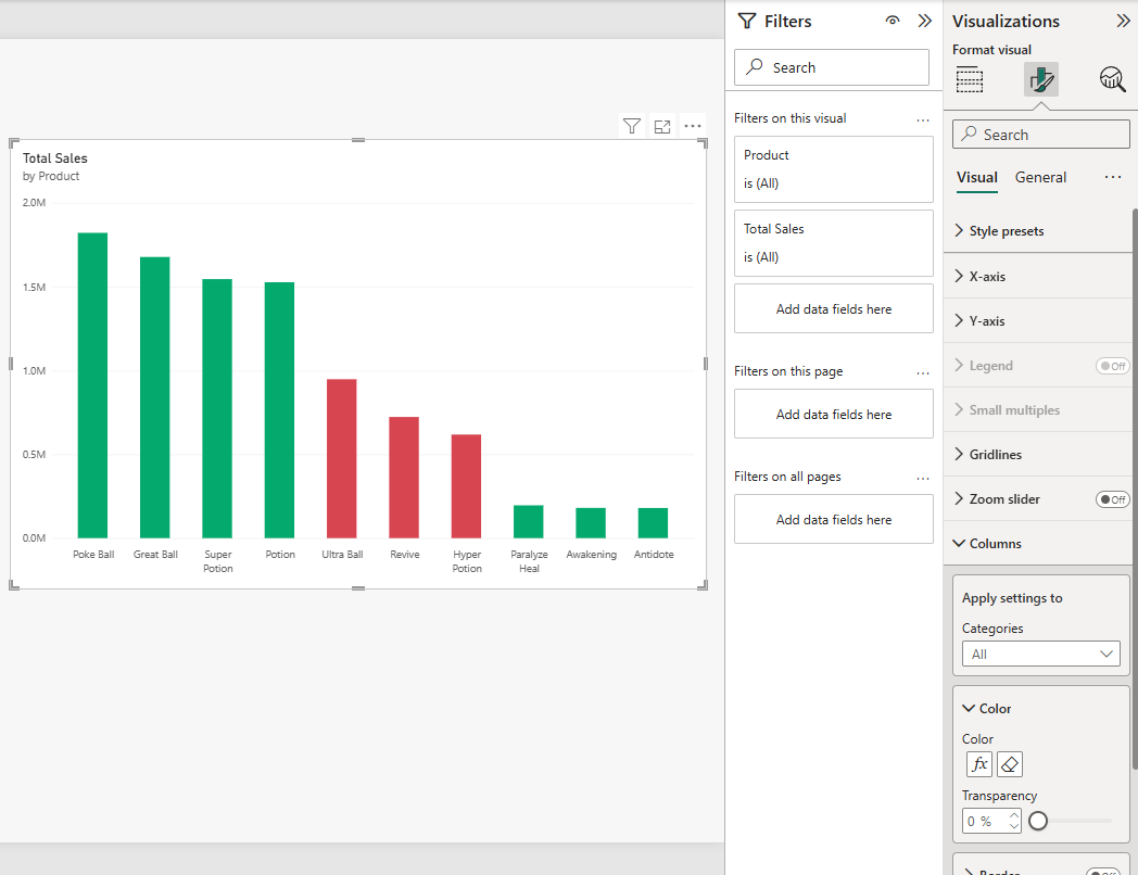
The three red columns sit together in the middle of the chart: mid-sized sales, but the lowest margins.
In the Columns section, the fx button opens the conditional formatting again, and the eraser button next to it removes it.
Remove Conditional Formatting
In a table or matrix, right-click the field in the Columns well, select Remove conditional formatting, and choose which kind to remove.
Note: Reset to default in the Format visual pane also removes conditional formatting rules.
Use it with care on a visual you have spent time on.
Good job! You have finished the Visuals chapter.
You can now build cards, KPIs, charts, slicers and formatted tables from your own Power BI model.
What's Next
Test what you learned with the Power BI Exercises.
This is the last chapter of the Power BI tutorial for now.
New chapters are on the way: Reports, where you turn your visuals into a finished report with several pages, and Sharing, where you publish the report to the Power BI service and share it with others.